This blog post describes the methodology to estimate solar power generation by all controlled premises with solar panels within a specific utility. Using this utility’s latitude and longitude, along with date and time, we can obtain reasonable forecasts of clear sky GHI, a measure of solar irradiance. In conjunction with cloud cover and the number of controlled premises with solar systems, we can use the following formula to create an estimate of solar generation:

\[Generation(kW)=units⋅5kW⋅\frac{GHI_{clearsky}(W/m^2)}{1000(W/m^2)}⋅[1−0.8⋅cloudCover]\]

Further explanation and pitfalls of this model are explored and discussed later in this post.

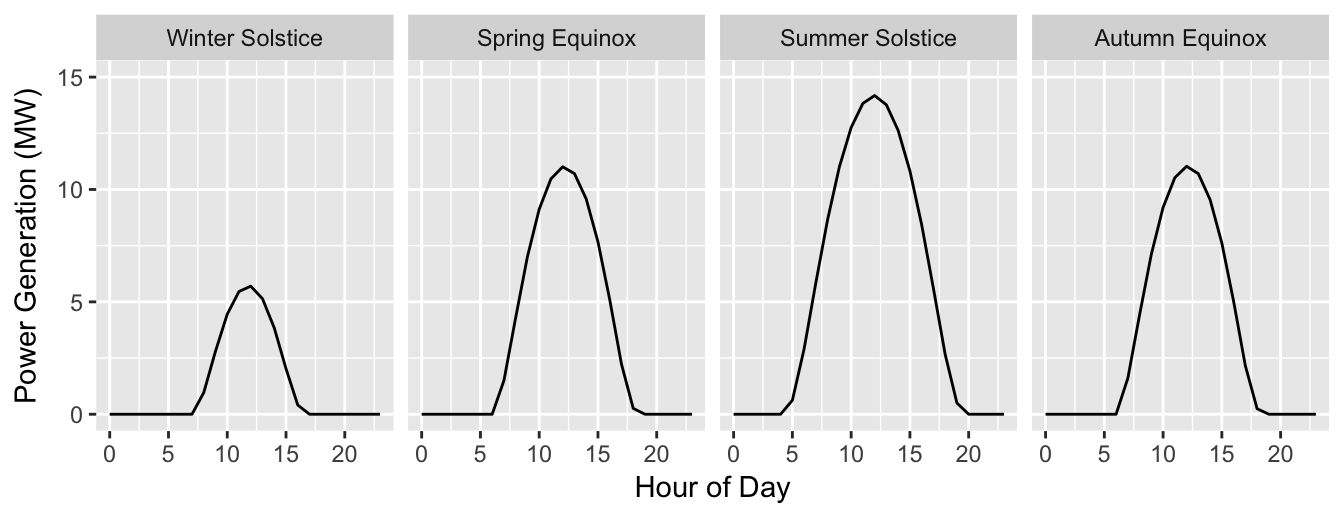
Example

A utility has informed us that they have roughly 15 MW of distributed solar generation capacity. If we assume 3000 units* of residential solar systems, we can obtain nearly 15 MW of power on the summer solstice from our calculation. Using the above formula and assuming clear skies, we observe the following power generation curves on the change of each season for 3000 units:

3000 units seems like a reasonable estimate for the number of distributed solar systems in our utility, as the population of the four cities it services was roughly 334,702 in 2015. Assuming a current population of 350,000 and 3 persons per household, this would make the penetration of solar around 2.6%, where 1.9% has been reported for the state of Colorado overall in 2016.

Introduction

Forecasting solar power generation can be a highly complex problem. In the long term, forecasts require a model to predict trends in solar system adoption by residences over time, as well as sophisticated models to predict typical atmospheric conditions for long forecast horizons (such as Numerical Weather Prediction).

For shorter forecast horizons, we rely on near-term forecasts of solar irradiance and atmospheric conditions. While sophisticated forecasts of irradiance can be purchased for a high price, simple formulas can be used in conjunction with cloud cover forecasts to generate reasonable forecasts of solar power generation.

Methods of Forecasting Solar Irradiance

Irradiance (W/m^2) is an instant measure of how much power reaches the earth from the sun over a fixed area at a specific point in time.

Insolatin (kWh/m^2) refers to the amount of total energy measured over the same fixed area for a specified amount of time.

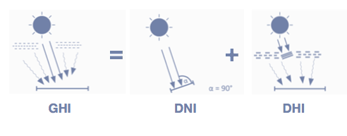
GHI is a useful measurement of solar irradiance, described as the amount of shortwave radiation recieved from above by a surface horizontal to the ground. It is measured by a horizontal pyranometer and accounts for both of the following measurements:

• Direct Normal Irradiance (DNI), the amount of solar radiation received by a surface held perpendicular to the rays of the sun (80% of GHI).
• Diffuse Horizontal Irradiance (DHI), the amount of radiation received by a surface that does not arrive directly from the sun, but rather from molecules and particles in the atmosphere (~20% of GHI).

The calculation of GHI using zenith angle alone is classified as a “very simple clear sky model”. When additional measurements of the atmospheric state are included, the model is upgraded to a “simple clear sky model”, and these typically include several atmospheric measures such as air pressure, temperature, humidity, site elevation, and more detailed cloud cover variables such as cloud type and height. Complex models take into consideration many additional atmospheric features such as Rayleigh scattering, aerosol measurements, and ground albedo.

(1) Using “Complex” GHI Models

Under this method, we would require forecasts of Global Horizontal Irradiance (GHI) from an external service such as Solargis, SolarAnywhere from Clean Power Research, or the Global Weather Corporation. Because cloud cover is embedded in measurements of GHI, additional cloud cover forecasts would not be necessary. This method unfortunately comes with a high price tag and all of the complications that arise when incorporating a new data source.

(2) Using “Very Simple Clear Sky” Models of GHI

We can develop a decent estimate of GHI using a very simple clear sky model and cloud cover forecasts.

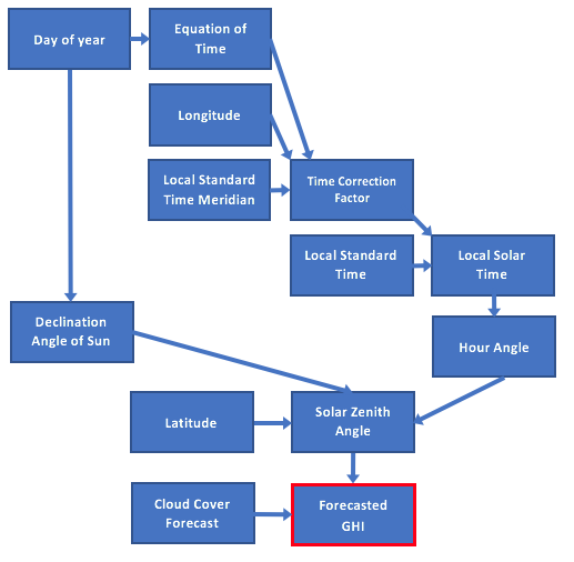
Full sun irradiance is derived from solar zenith angle, the angle between the sun and the vertical, which can be calculated using only latitude, longitude, date, and time. Solar zenith angle is calculated from these values alone and is based on all of the following sub-calculations:

• Equation of Time: angle based on the eccentricity of the Earth’s orbit and axial tilt.
• Time Correction Factor: Accounts for longitudinal variance within Local Solar Time.
• Local Solar Time: Time relative to the sun’s position in the sky - solar noon is when the sun is the * highest in the sky.
• Hour Angle: angle of the sun relative to the sun at solar noon.
• Declination Angle of the Sun: angle between the rays of the sun and the plane of Earth’s equator, which varies due to Earth’s axial tilt.

The Daneshyar–Paltridge–Proctor (DPP) model is used to convert solar zenith angle to an estimate of clear sky GHI:

\[GHIclear = DNI ⋅ cos(z) + DHI\]

where:

\[DHI=14.29+21.04(\frac{\pi}{2}−z)\] \[DNI=950.2(1−exp(−0.75(\frac{\pi}{2}−z)))\]

\(z\) = solar zenith angle

From here we can incorporate cloud cover forecasts to account for the impact of cloud coverage on GHI using a very basic formula:

\[GHI_{clouds} = GHI_{clear}⋅(1−0.8⋅cloudcover)\]

The measure \(.8⋅cloudcover\) is called cloud albedo and is defined as the amount of sunlight that reflects off the clouds back into space. On a perfectly clear day, there is no cloud albedo, but on an overcast day, 80% of solar radiation will reflect back into space.

Method Discrepancies

To investigate how well correlated observed GHI and estimated GHI are, we will use historical GHI from the National Solar Radiance Database (NSRDB) which utilizes the Physical Solar Model (PSM). Because the NSRDB only has publicly available data through 2015, we will will use data for the full year of 2015.

We only examine correlation for the hours between sunrise and sunset (when solar zenith angle < 90 degrees). The following plots show the relationship between estimated GHI (after incorporating cloud cover) and observed GHI, colored by hour of day and month of year:

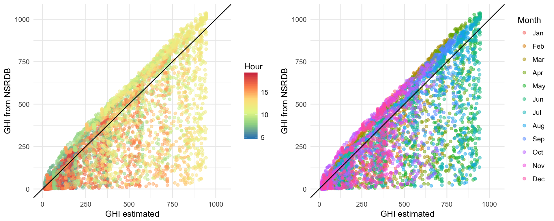
Figure 1: Scatter plots of forecasted versus true GHI, colored by time of day and month of year

The high concentration of points lying above the line of concordance implies that in these cases, the calculation of GHI slightly underestimates the observed GHI. This is likely due to the fact that the very simple GHI model does not account for site elevation.

However, calculated GHI often severely overestimates the true GHI. From the above plots, we can see that the largest discrepancies between estimated and true GHI tend to occur during peak solar hours (11 AM - 3 PM) and in peak solar months (May - August).

According to the documentation for the NSRDB, many additional factors are incorporated to the PSM which we are not able to account for with the Very Simple Clear Sky models:

> PSM uses a two-step process where cloud properties are retrieved using the adapted PATMOS-X model, which are then used as inputs to REST2 for clear sky and FARMS for cloudy sky radiation calculations. REST2 calculates both DNI and GHI. FARMS calculates GHI, and the DISC model is then used to calculate DNI. Aerosol properties are estimated using MODIS, MISR, and AERONET products. Water vapor is obtained from NASA MERRA. Additional meteorological parameters are also derived from MERRA.

While we would not be able to recreate the PSM model and derive perfect correlations, it appears we should be able to better predict true GHI with the addition of more cloud cover information, as evidenced by the following scatter plots:

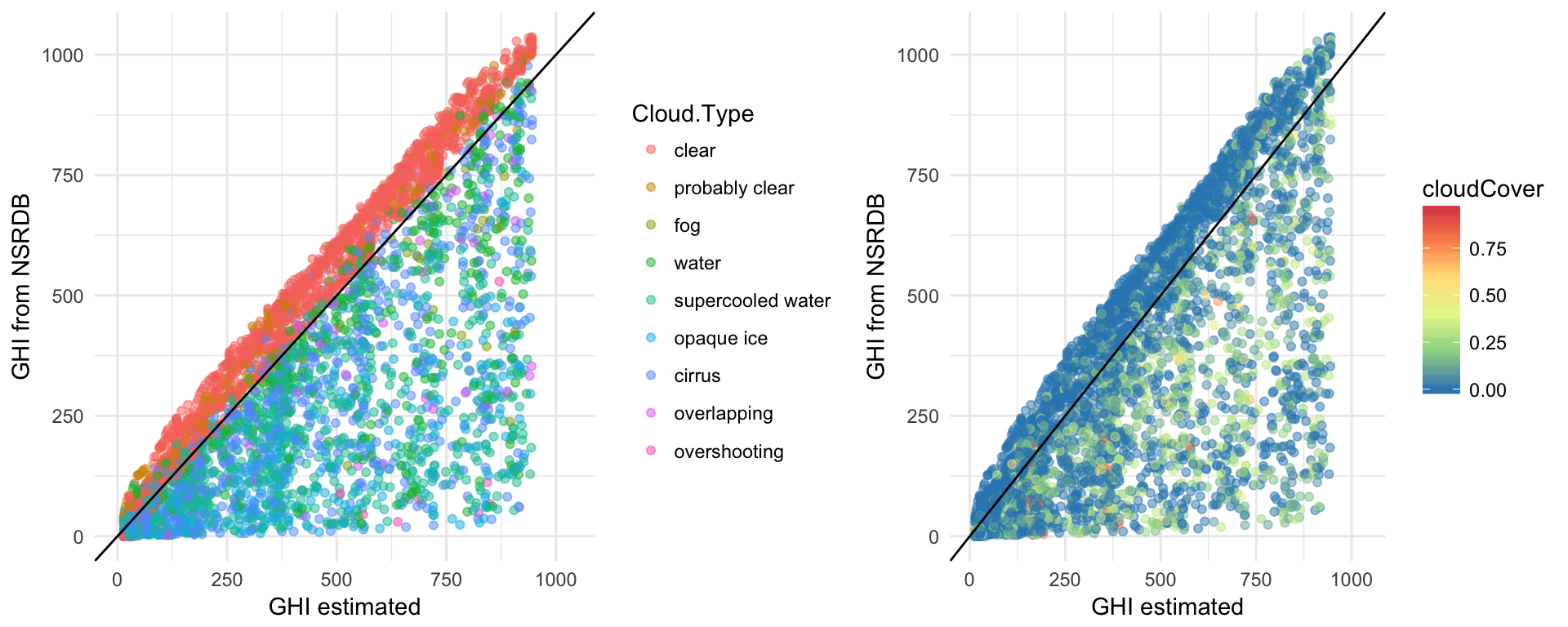
Figure 2: Scatter plots of forecasted versus true GHI, colored by cloud type (NSRDB) and cloud cover (Dark Sky)

We can see that Cloud.Type, as utilized by the PSM model and derived from NOAA’s PATMOS-x project for cloud algorithms, is much more predictive of the discrepancy between estimated and true GHI than Dark Sky’s historical cloudCover observations. Furthermore, there seems to be some disagreement between the two measures. As evidenced in the following boxplots, it appears within all the categories of cloud type except for “fog”, at least half of the observations were identified as 0% cloud cover from Dark Sky.

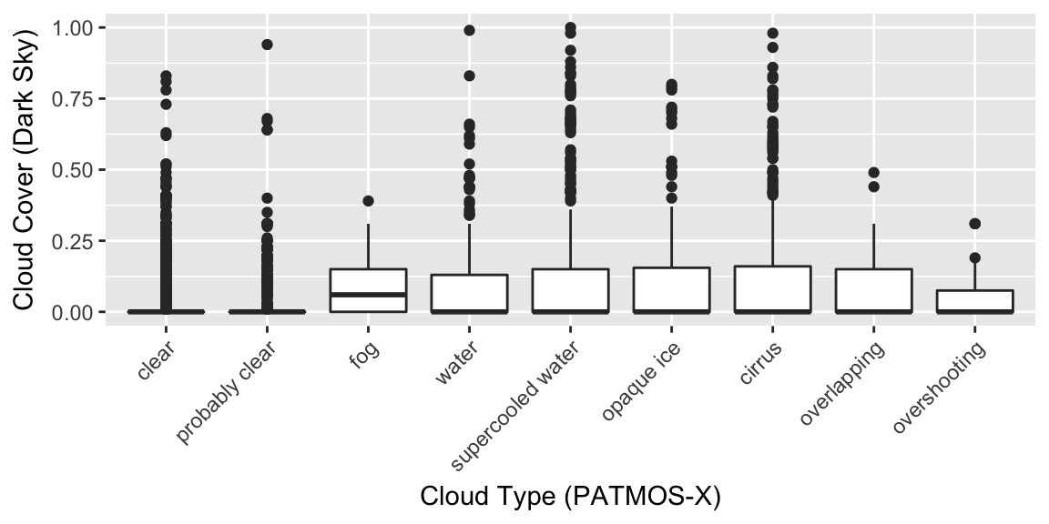
Figure 3: Boxplots of cloud cover (Dark Sky) by cloud type (NSRDB)

Reliability of Cloud Cover Forecasts The following histogram shows the distribution of hourly cloud cover observations in 2015 for our city as provided by Dark Sky:

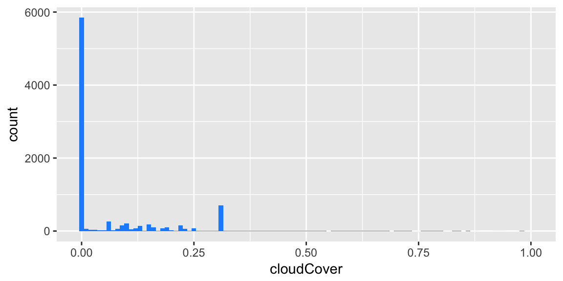
Figure 4: Histogram of Dark Sky cloud cover observations in 2015

Because so few hours (1.2%) are reported with cloud cover > 0.5 and because we see a value of 0.31 reported an artificially high proportion of the time (8.1%), it seems Dark Sky’s historical observations may not have been reliable in 2015, partially explaining the discrepancies in Figure 2.

However, for this project, the reliability of Dark Sky’s cloud cover forecasts are much more important. Fortunately, we have been pulling cloud cover forecasts and observations from Dark Sky for the past several weeks. From this, we can gauge (1) how reasonable the cloud cover forecasts seem, and (2) how the forecasts compared to the observations.

The following plot shows cloud cover observations as well as one-hour-out forecasts for a very cloudy start to autumn in Colorado. It is clear that cloud cover observations and forecasts, even those only one hour out, differ quite a bit.

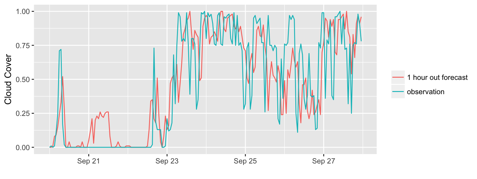
Figure 5: Comparison of Dark Sky observation and 1 hour out forecast during cloudy week in September 2017

If we expand the range of dates from when we started to pull data (around August 18, 2017 to September 27, 2017), we can observe the distribution of forecast error by forecast horizon:

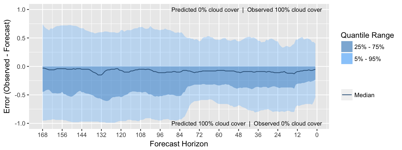
Figure 6: Distribution of Cloud Cover Forecast Error by Forecast Horizon

It appears cloud cover forecasts increase in reliability at around 72 hours out and again at around 12 hours out. In addition, it appears that at least 75% of forecasted values are larger than their resulting observations regardless of forecast horizon. This may indicate that Dark Sky uses a different model to generate forecasts than they use to report observations.

It is not possible to verify the accuracy of Dark Sky’s cloud cover observations with the data available. However, in the last 5 weeks we did not observe 0.31 appearing as frequently and values above 0.5 appear much more often (16.5%) than they did in 2015:

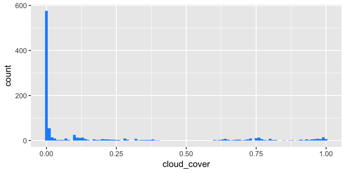
Figure 7: Histogram of Dark Sky cloud cover observations in August/September 2017

It is unfortunate the NSRDB does not report data for more recent time periods, as it would be useful to compare more recent Dark Sky cloud cover models against observed GHI. Because of this, it is difficult to determine whether another service would provide better forecasts of cloud cover than Dark Sky, or if cloud measurements beyond sky coverage would be critical to improving forecasts.

Mapping GHI to Power Generation

To properly convert GHI to power generation of all controlled residential premises with PV systems, we require information about the following:

• Average installed capacity under standard design conditions for a single PV system
• Standard design condition of PV system
• Number of controlled PV systems within a utility

Residential solar systems typically range in reported power output between 2 kW and 10 kW, but the most common system in the U.S. has a power output of 5 kW. A system with this capacity will generate 5 kW of power when irradiance is 1000 W/m^2, the standard design condition of PV systems. With the number of solar units within a utility, we can use the following equation to calculate total solar generation at any point in time.

\[Generation(kW)=units⋅5kW⋅\frac{GHI(W/m^2)}{1000(W/m^2)}\]

Recall, GHI has already factored in cloud cover:

\[GHI_{clouds}=GHI_{clear}⋅(1−0.8⋅cloudCover)\]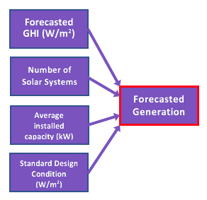

Additional Considerations

While GHI and cloud cover forecasts are the single most important measurements to forecasting solar power generation, there are several other factors that could be included to improve forecasts:

• Clear sky GHI does not account for tilt angle of panels. Because GHI is a measure of solar insolation on a flat panel, solar generation forecasts would increase if we are able to account for tilt angle.
• Clear sky GHI does not account for elevation. The formulas utilized to calculate GHI assume a location at sea level, and will bias forecasts low for higher elevations.
• Solar panels begin to lose efficiency at warmer temperatures. If temperature was built into the forecast model, solar generation forecasts would decrease on hot days.
• The most sophisticated GHI predictions distinguish between clouds at varying levels and of various types, not just total cloud cover. Such models also incorporate atmospheric aerosols and other pollutant information. In cases of severe pollution, solar power generation can be reduced by up to 20%.

References

https://nsrdb.nrel.gov

http://www.ammonit.com/en/wind-solar-wissen/solarmessung/473-measuring-sun-radiation

http://energy.sandia.gov/wp-content/gallery/uploads/SAND2012-2389_ClearSky_final.pdf

http://ieng6.ucsd.edu/~dplarson/LarsonNonnenmacherCoimbra2016.pdf

http://www.sciencedirect.com/science/article/pii/S0196890413001039

https://www.ohmhomenow.com/2016-solar-penetration-state/

Monforte, F. A., Dr., Director of Forecasting Solutions. Forecast Practitioner’s Handbook: Incorporating the Impact of Embedded Solar Generation into a Short-term Load-Forecasting Model. Itron, Inc.